High-level cctbx objects: models, maps, reflection data, symmetry and arrays
Introduction
In cctbx you often work with objects that represent the things you are interested in: models, maps, reflection data, symmetry and so on. For example, you might create a model object that represents a 3D structure of a protein and a map object that represents a 3D cryo-EM map. Then you carry out operations using these objects. For example you might refine the model against the map data.
The principal high-level cctbx objects are:
- DataManager: Read and write files and keep track of them
- model_manager: A 3D model or models and restraints that go with them
- map_manager: A 3D map or maps and information about gridding and map symmetry
- map_model_manager: One or more maps and models as a group
These high-level cctbx objects are made up of lower-level objects that represent arrays of different kinds and that represent features such as symmetry. The importance of these lower-level cctbx objects is that they have many packaged methods that can carry out standard operations on their data. For example, a linear (flex.double) array has a standard_deviation_of_the sample method that calculates the standard deviation of the values in that array.
Some important slightly lower-level cctbx objects are:
- flex_array: Array containing data of any kind. These can be linear arrays or multi-dimensional arrays
- miller_array: One 3D Fourier representation of a map (map coefficients) or other data such as a weight for each index of a map
- crystal_symmetry: Symmetry information about a map, model or fourier representation
- ncs_object: Symmetry that is not crystallographic. For example, symmetry of a cryo-EM map or symmetry of a model
Each of these objects is described below along with some examples of how they are used. You can cut and paste the examples provided to see how they work or to create your own code. We’ll start by generating a map and model.
Start Python from cctbx, generate a model and a map
First let’s start up python from cctbx so that it knows about all the cctbx modules. You can just type all the commands specified here in a terminal window to do everything described below. Type this into your terminal window to start python:
libtbx.python
Note that you used libtbx.python and not python. If you have installed cctbx, then the libtbx.python command runs a version of python that is compatible with cctbx and that already knows about cctbx so that you can import cctbx functions easily.
Let’s create a map file and a model file and some Fourier coefficients so that we can work with them later. There is a tool to create a dummy model and map available in the map_model_manager.
Let’s create a map_model_manager and call it mmm (you can call it whatever you want, mmm is just short for map_model_manager):
from iotbx.map_model_manager import map_model_manager      # load in the map_model_manager
mmm=map_model_manager()     # get an initialized instance of the map_model_manager
Notice that the text following the hashtag is ignored. These are comments that you can include in Python code; they can help a reader understand what the code is supposed to do.
Right now, the map_model_manager object is an empty container. To be useful, we need to have a model and a map. In production, this will be typically done by setting up our map_model_manager object with map and model objects. But it is also possible to get a model from cctbx example structures, and to calculate a map from that model. For simplicity, let’s use a model from the cctbx examples. The method generate_map() will do both, obtaining the model from the examples and calculating a map from it:
mmm.generate_map() # get a model from a small library model and calculate a map for it
The generate_map() method has many options that let you choose model parameters (such as the number of residues (n_residues), or the B-factor (b_iso) and map parameters (such as the high resolution limit (high_resolution) and the scattering table (scattering_table)). It is also possible to supply a model file (“model_file_name”). Note that the default choice for the scattering table is “electron”, so it will create a cryo-EM map. If you want an electron density or nuclear density map, the value will have to be modified accordingly. Let’s write out the map and model we just created:
mmm.write_map("map.mrc")     # write out a map in ccp4/mrc format
mmm.write_model("model.pdb")     # write out a model in PDB format
Now we have a model and a map that we can work with, written out as files to model.pdb and map.mrc so we can read them in at any time. If you have a visualization tool like Coot or ChimeraX, you can look at the map and model and see that the map looks like an outline of the model.
The map_model_manager can take a model fragment from cctbx examples and calculate a map for it. The image below shows the example model and map obtained using default options for the generate_map() method. The model represents a small helical fragment.
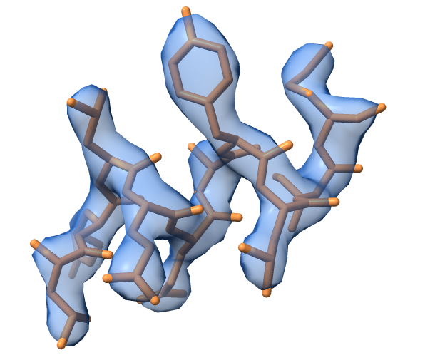
Tip: Change the values for high_resolution or b_iso and have a look how the calculated map changes. It can be also interesting to change the scattering table.