Working with models: the cctbx Model manager

Learn how to use the cctbx model manager. It lets you do some basic operations on models. This tutorial shows how to set up the model manager, apply coordinate shifts, do atom selections and calculate model-based map coefficients.

Representing a macromolecular structure

A macromolecular structure is usually represented by a model manager object in cctbx and is typically called a “model”. A model usually consists of one or more chains - polypeptide chains for a protein, nucleic acid chains for DNA or RNA - with chain names like chain A, chain S etc. Each chain is composed of a series of amino acid or nucleic acid residues, such as leucine for protein or guanine for RNA, with each residue having a name and a number. Each residue constitutes a set of atoms, for example N, CA, C, O for the main chain of a protein. Then for each atom, the model normally contains values of its coordinates (x, y, z), a B-value (atomic displacement parameter), and an occupancy (zero to one). There may be additional parameters describing an atom, such as anisotropic B-values.

There may also be ligands, water molecules, and other coordinate information represented in a model object. These are typically called “heteroatoms” to differentiate them from the “atoms” of the protein or nucleic acid.

The model object - more than the atomic description

In addition to the description of atomic contents of a structure, a model object contains information about the size of the box in which the model placed. This box corresponds, for a cryo-EM structure, to the box of density in the reconstruction. For a crystal structure the box is the unit cell (smallest unit repeated by translations) of the crystal. This box is usually represented as a “crystal_symmetry” object containing the symmetry of the box of density (P1, or no symmetry for cryo-EM, any crystallographic symmetry for a crystal structure), and also containing the dimensions and angles of the box. A map and a model, each representing the full box, normally will have the same crystal_symmetry object representing them.

The model object also may contain information about the geometrical restraints to be applied to the model coordinates. These may include expected distances between atoms, bond angles and torsion angles. They may also include information about the relationship between the coordinates in this model and some other reference structure, or between different parts of this model that are related by symmetry within the molecule.

File types that store models

The most commonly used file types to store a macromolecular model are the 'mmCIF' and the 'PDB' format. Both are text files that can be opened in a text editor. The PDB format can be easily read by eye, as the information is arranged in fixed format columns. The mmCif format is hard to read by eye and must usually be interpreted by software. As the mmCIF format is more general, it has replaced the PDB format for "official" use, such as in the Protein Data Bank. However, PDB files can be still used by many programs and it is useful for illustrating the concepts of a model. For this reason, the cctbx documentation will often use PDB files as example.

An example for a simple model

Below is simple model in PDB format:

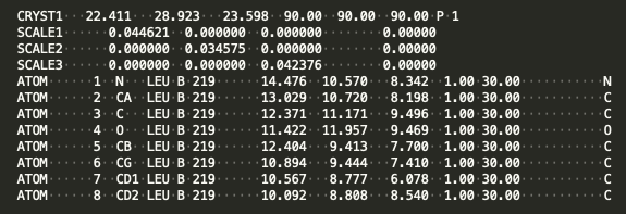
This model represents a leucine residue in a P1 unit cell. The CRYST1 line gives the cell dimensions (22.411, 28.923, 23.598) in Angstroms, the cell angles (90, 90, 90) in degrees, and the space group (P1, or no symmetry). The SCALE lines give the relationship between cartesian coordinates and fractional coordinates. The ATOM lines consist of an atom number (1-8 in this example), atom names (N, CA, etc), residue name (LEU), chain ID (B), residue number (219), coordinates (e.g., (14.476, 10.570, 8.342)), the occupancy of each atom (fraction of time this atom is thought to be present, from zero to one), and B-value (30.00, a measure of how variable the position of this atom is). The last characters in the line represent the element of the atom (N, C, O etc).

This simple (PDB) representation is sufficient to define many aspects of a model and can be recognized by the model manager. The mmCIF representation has more flexibility but generally contains the same information.

Setting up an example model

The cctbx model manager lets you view and change many attributes of a model. Let’s work with a library model that we can obtain with the map_model_manager (revisit this page if you need a refresher on high level objects):

from iotbx.map_model_manager import map_model_manager      #   load in the map_model_manager
mmm=map_model_manager()         #   get an initialized instance of the map_model_manager
mmm.generate_map()              #   get a model from a small library model and calculate a map for it
mmm.write_map("map.mrc")        #   write out a map in ccp4/mrc format
mmm.write_model("model.pdb")    #   write out a model in PDB format

Then we will set up the DataManager and read the example model (described here):

from iotbx.data_manager import DataManager    #   Load in the DataManager
dm = DataManager()                            #   Initialize the DataManager and call it dm
dm.set_overwrite(True)         #   tell the DataManager to overwrite files with the same name
model_filename="model.pdb"                         #   Name of model file
model = dm.get_model(model_filename)               #   Deliver model object with model info

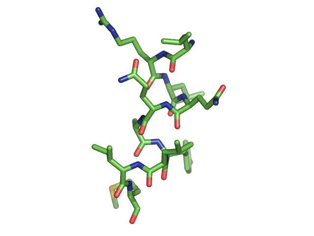
Below is a figure of the model. It represents a short helical fragment.

Accessing attributes of a model with the Model manager

Now let’s get an array containing the coordinates of the atoms in our model:

sites_cart = model.get_sites_cart()          #      get coordinates of atoms in Angstroms

We can look at the value of the first coordinate in this list (x, y, z):

print (sites_cart[0])     #    coordinates of first atom

This yields:
(14.476000000000003, 10.57, 8.342)

Notice that these are the same values that were on the first line of the PDB representation of this model:

There are many things you can do with a model. The fundamental one is that you can change the coordinates. We’ll use a little tool called “col” to allow us to add the coordinate shift (1,0,0), adding +1 Angstrom in X, to all the coordinates in the model:

sites_cart = model.get_sites_cart()          # get coordinates of our model
from scitbx.matrix import col                # import a tool that handles vectors
sites_cart += col((1,0,0))                   # shift all coordinates by +1 A in X
model.set_sites_cart(sites_cart)             # replace coordinates with new ones
print (model.get_sites_cart()[0])            # print coordinate of first atom

This yields:
(15.476000000000003, 10.57, 8.342)

We can write out or shifted model and see that it has shifted from its original position:

dm.write_model_file(model, "shifted_model.pdb", overwrite=True)

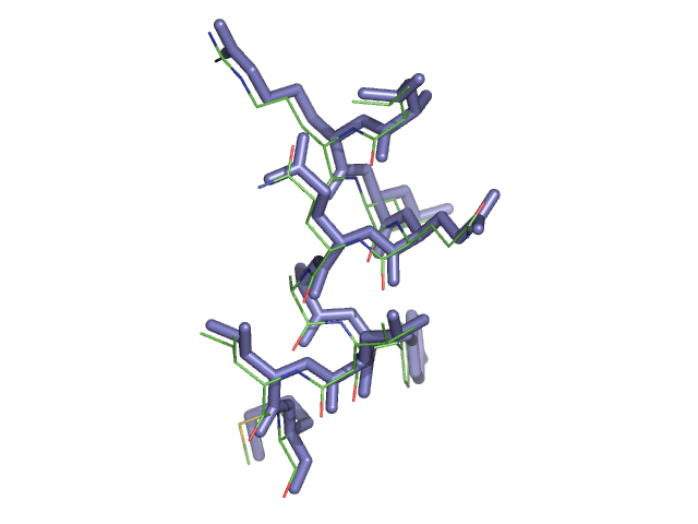
Below is a figure showing the initial model (shown as lines) and the shifted model (blue stick representation).

Atom selections with the Model Manager

Sometimes you want to perform action on parts of a model. The cctbx model manager lets you create a new model containing only a selected part of your current model. This is a really powerful feature. Let’s select a few parts of our model and work with them. First let’s get a clean copy of our model by loading the initial file (model.pdb):

model_filename="model.pdb"                         #   Name of model file
model = dm.get_model(model_filename)               #   Deliver model object with model info

The model contains residues from 219 to 228, but how would we know this without looking at the model in a viewer or in a text editor? Let’s see how we could find out what residues are in this model by selecting all the atoms named “CA” and printing them out (here CA is one of the 4 protein main-chain atoms which are N, CA, C, O):

sel =  model.selection("name CA")     # identify all the atoms in model with name CA

The selection array sel is a one-dimensional array with one value for each atom in the model (i.e. if the model has n atoms, the array has length n). Each value is either True (keep this atom) or False (do not include this atom). Next we create a new model, selecting atoms based on the sel selection object:

ca_only_model = model.select(sel)     #  select atoms identified by sel and put in new model

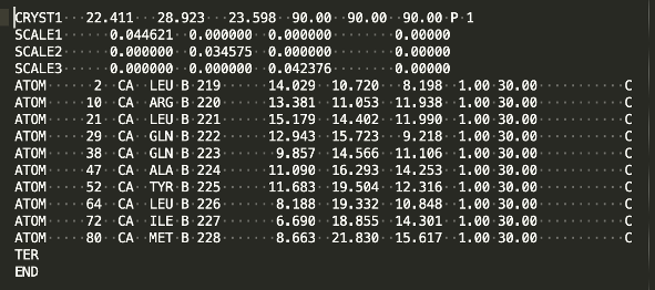
Now ca_only_model is a new model that contains a piece of the original model object. In this case it contains all the atoms with the name “CA”. Let’s print it in PDB format to see what residues are present:

print (ca_only_model.model_as_pdb())      #  print out the CA-only model in PDB format

We can save the new model in a PDB file too:

dm.write_model_file(ca_only_model, "ca_model.pdb", overwrite=True)

There are many things you can use as selections. For example, you can select all the residues from 219 to 223 in chain B with the selection string "chain B and resseq 219-223". You can find more information on selections in the Phenix documentation about atom selections.

Creating model-based map coefficients

The cctbx model manager contains nearly all the information necessary to generate model-based map coefficients. Let’s create some map coefficients from our model. First let’s get a fresh instance of our model:

model_filename="model.pdb"                         #   Name of model file
model = dm.get_model(model_filename)               #   Deliver model object with model info

Now let’s use that model, along with its symmetry information, to generate map coefficients. We’ll use a tool that is found in cctbx.development.create_models_or_maps called generate_map_coefficients that makes it easy to get map coefficients from a model:

from cctbx.development.create_models_or_maps import generate_map_coefficients   # import the tool

map_coeffs = generate_map_coefficients(  # generate map coeffs from model
      model=model,                       # Required model
      d_min=3,                           # Specify resolution
      scattering_table='electron')       # Specify scattering table

Note that we have to set the high-resolution limit (d_min = 3 Angstroms) and tell the tool whether we are working with cryo-EM (scattering_table='electron') or X-ray (scattering_table='n_gaussian'). We can use these map coefficients to calculate a map, or use them directly for some other purpose. Let’s make a map using these map coefficients:

from cctbx.development.create_models_or_maps import get_map_from_map_coeffs   #  import the tool
map_data = get_map_from_map_coeffs(map_coeffs = map_coeffs)   #  create map from map coeffs

Here the array map_data corresponds to the map data (not a map_manager object). Note that this map will be on a grid that is automatically chosen. If you want to specify the grid, you can use the keyword n_real, for example n_real=(36,27,95).

If you already have a map_manager object mm and you want this map to match that map_manager, you can use the map_manager object to calculate map_data and put it in a new map_manager matching the current one:

# mm_model_map= mm.fourier_coefficients_as_map_manager(map_coeffs)   # generate map from map coeffs