HKLViewer tutorial
This tutorial shows some use cases of the HKLviewer.
Display I/SigI of a dataset
Reflections with I/SigI > 2 are considered to be good data for structure solution. Therefore, this cutoff is often used to determine the resolution limit. Here we examine a problematic dataset to show that for a given threshold of I/SigI a matching resolution cutoff does not necessarily exist.
Open the dataset merged.mtz in the HKLviewer. The IMEAN,SIGIMEAN reflections are shown by double clicking the row with that label in the upper left table.
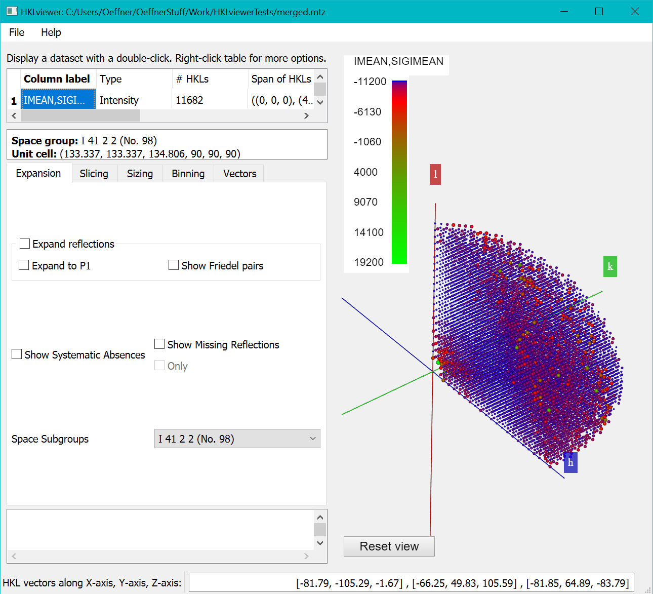
By default, the colour mapping for each reflection is according to values of the intensity. The next section explains how to color according to I/sigI values.
Computing I/SigI
Right click the row with the "IMEAN,SIGIMEAN" label and from the context menu select “Make a new dataset from this dataset and another dataset”.
In the “Create New Reflection data” dialog enter the lines of python code as given below into the textbox and “IoverSigI” as the formula and the label for the new data respectively.
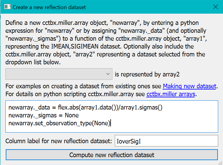
The first statement newarray._data = flex.abs(array1.data())/array1.sigmas() computes the I/SigI of all data values but with the absolute values of the intensities since there appear to be a significant number of negative intensities.
For convenience newarray is initialised to a copy of the original array (here representing "IMEAN,SIGIMEAN").
For I/SigI data we are not interested in the sigma values themselves. So we discard the sigmas array with the second statement newarray._sigmas = None.
The third statement newarray.set_observation_type(None) is optional. It tells CCTBX to deduce which type of data newarray will contain. In the case of I/SigI it will be plain real numbers. It could have been more specialised types such as map coefficients or X-ray observations. Since the colour mapping and sizing schemes are specific to each observation type, datasets classified with sensible observation types makes it easier to compare datasets in the viewer with other datasets of the same observation type.
Clicking the "Compute new reflection dataset" button will execute the script and display the IoverSigI dataset in the viewer as below
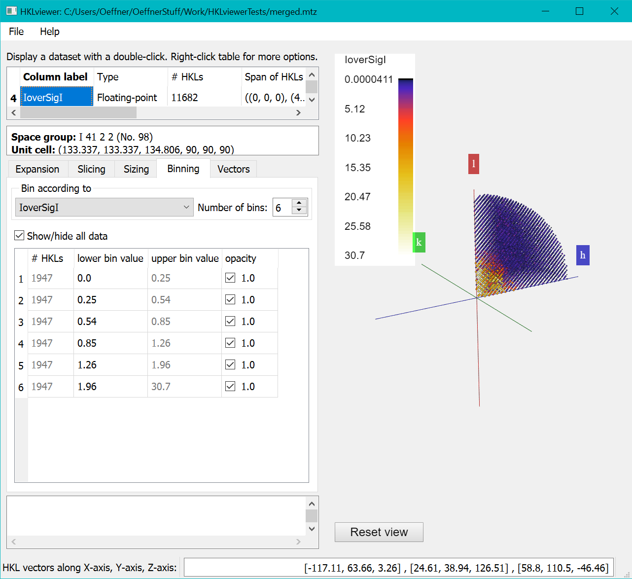
The "Binning" Tab lets you choose the number of bins and the thresholds. By default data is binned according to resolution.
But here we have binned against the newly created “IoverSigI” column and set the number of bins to 6.
HKLviewer will try to put an equal number of reflections into each bin and then compute corresponding bin thresholds. For this exercise,
we want the bin thresholds at defined I/SigI values: 4.0, 3.0, 2.0 and 1.0.
Do this by entering these new bin thresholds by typing the numbers 4,3,2,1 in row 6, 5, 4 and 3 in the “lower bin value” column.
Then untick the "Opacity" checkboxes of the first three bins to hide reflections with I/SigI less than 2.
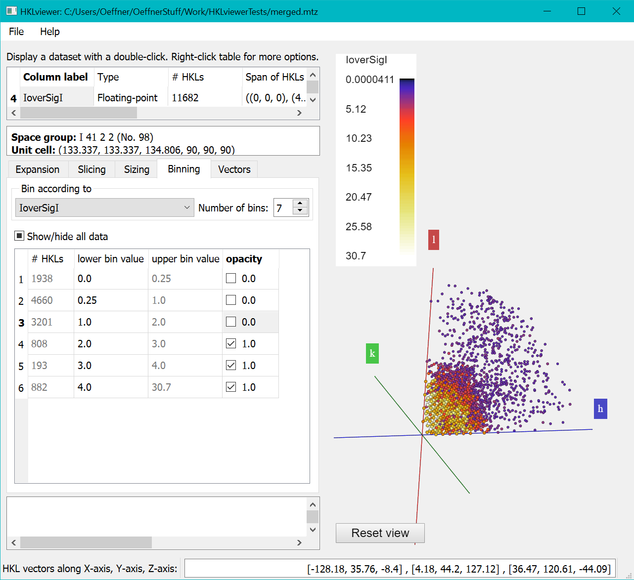
The first column of the "Binning" shows the number of reflections in each bin. The relatively small total number of reflections with I/SigI > 2 suggests that it could be difficult to solve the structure for this data set. This is also visible in the Viewer on the right, which shows much fewer spheres than the figure above where none of the bins have been excluded.
Inspecting TNCS modulation in a dataset
tNCS or pseudo-symmetry is a crystal pathology where two or more molecules in the unit cell are aligned in a way to cause interference in the diffraction pattern.
It shows as periodic modulation of the diffraction pattern and can cause problems for structure solution unless identified and taken into
account by the software. tNCS vectors are real space vectors and can be determined before structure solution attempts.
The dataset 6C5F (available from the PDB) has tNCS which is detected by programs such as phenix.xtriage.
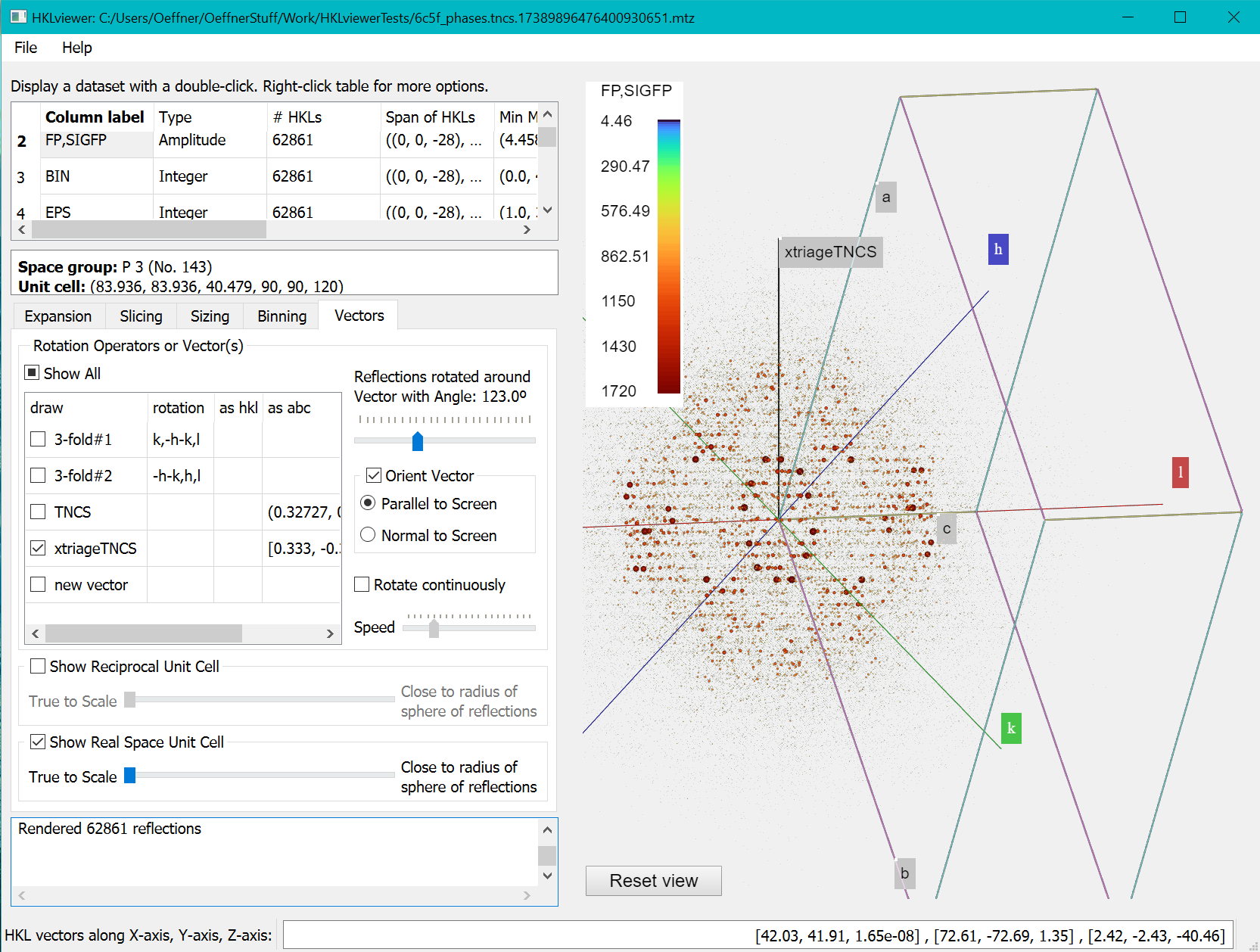
It determined the pseudo-symmetry vector to be [0.333, -0.334, 0.040] in fractional coordinates. Follow the steps below:
- Open the data file in the HKLviewer.
- Double click the "F_meas_au,F_meas_sigma_au" label (or "FP,SIGFP" if loading an mtz file) to display the data.
- On the Expansion tab, expand the reflections to a sphere.
- On the sizing tab, tick the “User defined power scaling” checkbox and enter a power factor of 2 to obtain values that are roughly proportional to intensities (the file from the PDB does not provide the original intensity data).
- On the Vectors tab, enter the coordinates for the tNCS vector found by xtriage [0.333, -0.334, 0.040] on the last line by overwriting the “new vector” label to “xtriageTNCS” and entering the coordinates in the same row under the “as abc” column. Pressing return will submit the vector to HKLviewer.
- Tick the xtriageTNCS vector checkbox as well as the “Orient vector” checkbox and the radio button “Parallel to screen”.
- Either rotate the reflections manually on the slider control or tick the “Rotate continuously” checkbox.
This will show the modulations in the data as ripples in the reflections in planes perpendicular to the tNCS vector. It can be useful to tick the “Show Real Space Unit cell” checkbox to see where the tNCS vector points within the unit cell.
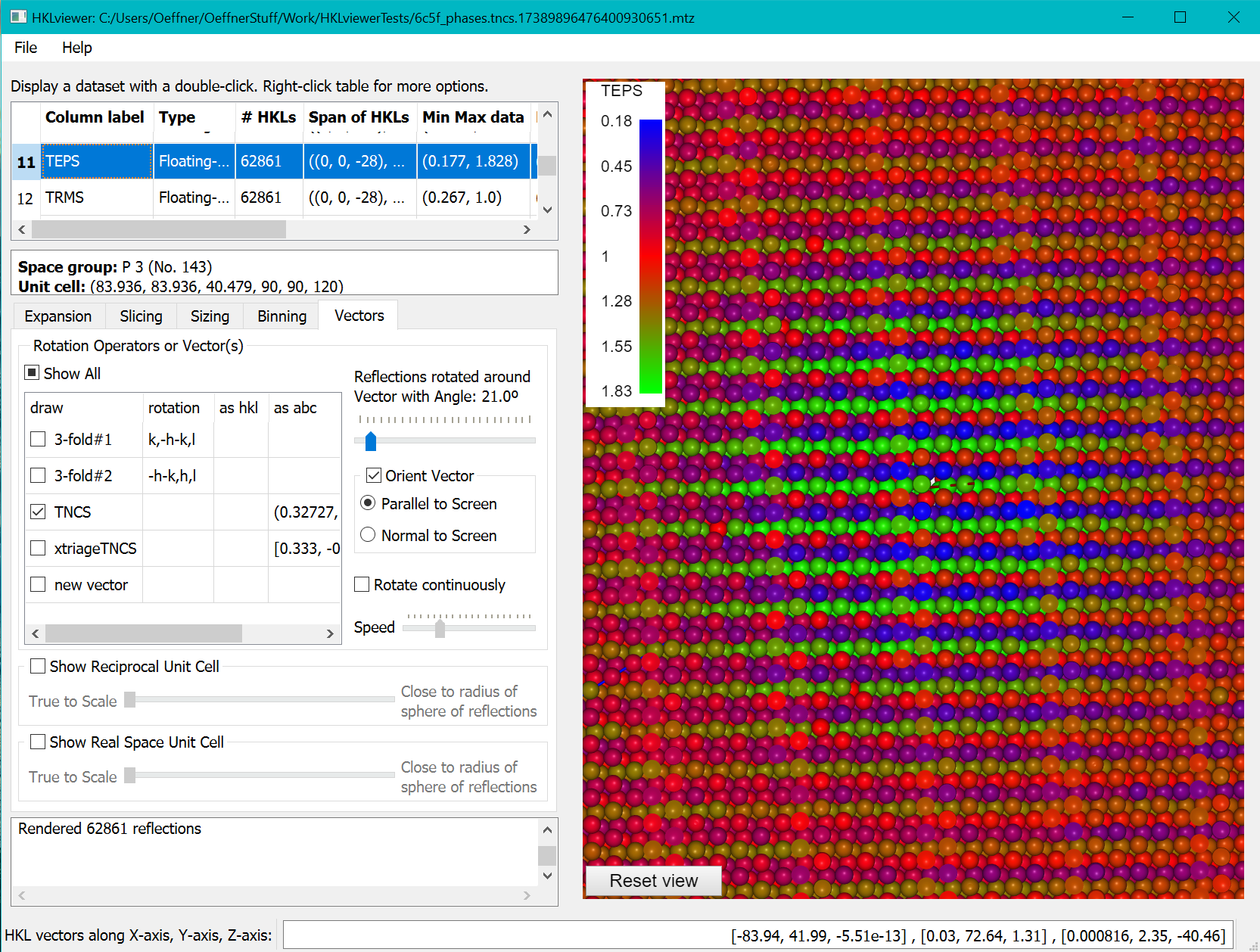
Phasertng, which is currently under development, stores a data column, TEPS, with the correction factors, epsilon, revealing the tNCS modulation of the intensities. The coordinates for the tNCS vector is embedded in the mtz file when the mtz file has been processed with phasertng. This is illustrated below where the reflections have been sliced with a clip plane width of 8. On the sizing tab we have set the power factor to 0 and the linear scaling factor to 0.8. The modulation is clear from the alternating layers of red, green and blue layers of reflections.
Inspecting a twin law
The phenix tutorial with the file, porin.mtz, illustrates twinning. The twin operator found by phenix.xtriage is -h-k,k,-l.
Follow the steps below:
- Load the file in the HKLviewer and display the dataset “F-obs,SIGF-obs”.
- On the Vectors tab, enter the twin operator into the table of vectors; first by overwriting the last row with the “new vector” string with “twin”. Then by entering the string “-h-k,k,-l” in the adjacent rotation column and pressing return for the HKLviewer to accept the new twin operator. It turns out to be a 2-fold rotation so the HKLviewer will prefix the name with 2-fold.
- Press the “Orient vector” checkbox and the radio button “Normal to screen”.
- On the Expansion tab, expand the reflections to P1 and Friedel mates.
- On the Slicing tab, tick the “Slice with a clip plane” checkbox and set “Distance from Origin” and “Clip plane width” to 4 and 1 respectively.
- Show a “Tabulated Reflection data” window by right clicking the column label “F-obs,SIGF-obs” in the upper left table and selecting “Show a table…” from the menu.
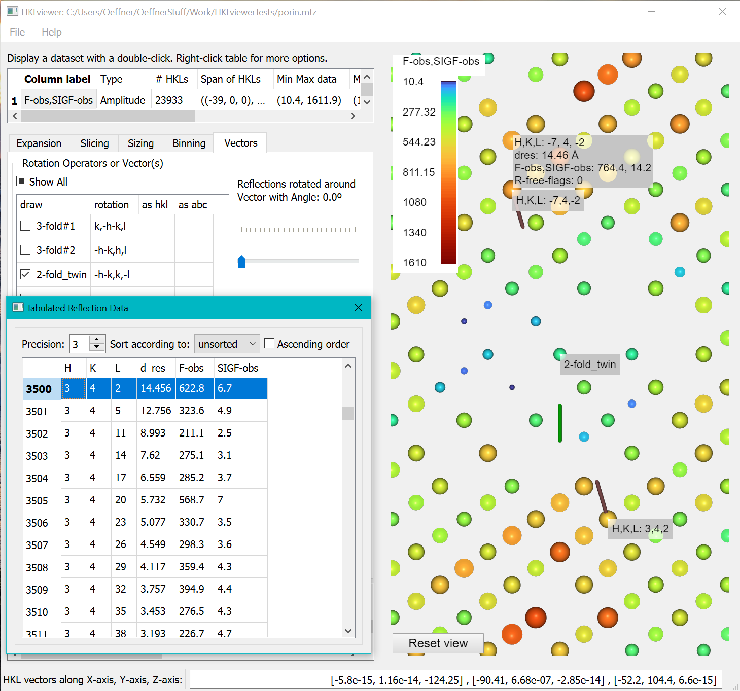
To inspect data values of reflections related by the twin operator right-click a reflection in the view. It will bring up two tooltips with the hkl indices at the end of two vectors from the reciprocal space origin pointing to the twin reflections. Due to the clip plane, the vectors may not be fully visible. Double click one of the reflections to bring up the standard tooltip with all other values represented by this reflection (dres, F-obs, SIGF-obs, R-free-flags). Right-clicking a reflection will highlight the data value in the “Tabulated Reflection data” window. The HKL indices in the table are the original from file. Since the twin operator is not part of the spacegroup the hkl index in the tooltip of a twin related reflection may differ from the HKL index generated by P1 or Friedel mates expansion highlighted in the Tabulated Reflection Data.